Contents
Double Integrator Reach-Avoid Via Dynamic Programming
This example will demonstrate the use of SReachTools to solve a terminal-hitting time stochastic reach-avoid problem using dynamic programming. We consider a stochastic continuous-state discrete-time linear time-invariant (LTI) system. This example script is part of the SReachTools toolbox, which is licensed under GPL v3 or (at your option) any later version. A copy of this license is given in https://sreachtools.github.io/license/.
In this example, we analyze the following problems via dynamic programming for a stochastic system with known dynamics:
- stochastic viability problem: Compute a controller to stay within a safe set with maximum likelihood
- the terminal-hitting time stochastic reach-avoid problem: Compute a controller that maximizes the probability of reaching a target set at a time horizon, N, while maintaining the system in a set of safe states
- stochastic reachability of a moving target tube: Compute a controller that maximizes the probability of staying within a target tube (a collection of time-varying safe sets)
SReachTools has a dynamic programing implementation that can analyze systems upto three dimensions. For efficient implementation, we require the input set to be an axis-aligned hypercuboid, and define the grid the smallest hypercuboid containing all the target sets.
% Prescript running: Initializing srtinit, if it already hasn't been initialized
close all;clearvars;srtinit;
Problem setup
In this example we use a discretized double integrator dynamics given by:
![$$ x_{k+1} = \left[ \begin{array}{cc} 1 & T \\ 0 & 1 \end{array}\right]
x_{k} + \left[\begin{array}{c} \frac{T^{2}}{2} \\ T \end{array}\right]
u_{k} + w_{k}$$](dIntSReachDyn_eq10500098239847735597.png)
with state  , input
  , disturbance
  , and sampling time
  .
.
The double integrator system can be used as a simple model of a vehicle on a lane.
- The state is position and velocity of the vehicle.
- The vehicle is acceleration-controlled with restrictions on the maximum and minimum acceleration provided
- The stochastic disturbance affects its position and velocity accounting for unmodelled phenomena like slipping or engine model mismatch.
% System definition
% -----------------
% discretization parameter
T = 0.1;

% define the system
sys = LtiSystem('StateMatrix', [1, T; 0, 1], ...
    'InputMatrix', [T^2/2; T], ...
    'InputSpace', Polyhedron('lb', -0.1, 'ub', 0.1), ...
    'DisturbanceMatrix', eye(2), ...
    'Disturbance', RandomVector('Gaussian', zeros(2,1), 0.01*eye(2)));

% Parameters for dynamic programming and visualization
% ----------------------------------------------------
% Step sizes for gridding
dyn_prog_xinc = 0.05;
dyn_prog_uinc = 0.1;

% Additionally, we need to specify thresholds of interest to compute the
% stochastic viability set
reach_set_thresholds = [0.2 0.5 0.9];

% For plotting purposes, we specify legend and axis limits
axis_vec = [-1 1 -1 1];
legend_str={'Safety tube at k=0', 'Safety Probability $\geq 0.2$', ...
    'Safety Probability $\geq 0.5$', 'Safety Probability $\geq 0.9$'};
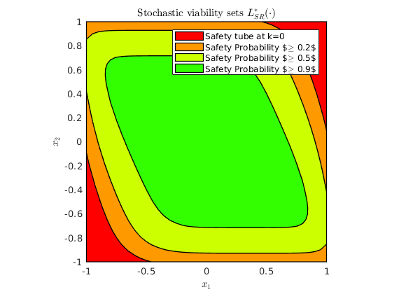
Case 1: Stochastic viability problem
We are interested in assessing the safety of this double integrator system to stay within the safe set of ![$[-1,1]^2$](dIntSReachDyn_eq04712238727479698605.png) .
.
For the vehicle in a lane example, we require controllers that maximize the probability of ensuring that the position stay within ![$[-1,1]$](dIntSReachDyn_eq01893875229900969577.png) and the velocity with when the car at
and the velocity with when the car at  has some initial position and velocity in .
To perform this safety analysis, we need to do the following steps
- Provide parameters for dynamic programming like grid size and thresholds (if stochastic viability sets are of interest) [*Reused from above*]
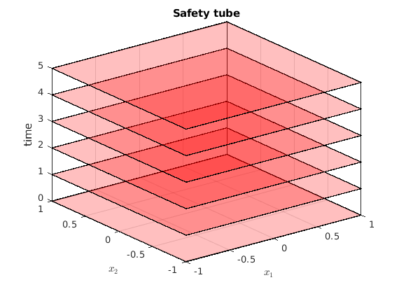
- Construct the safety tube using 'viability' option (and plot it as well)
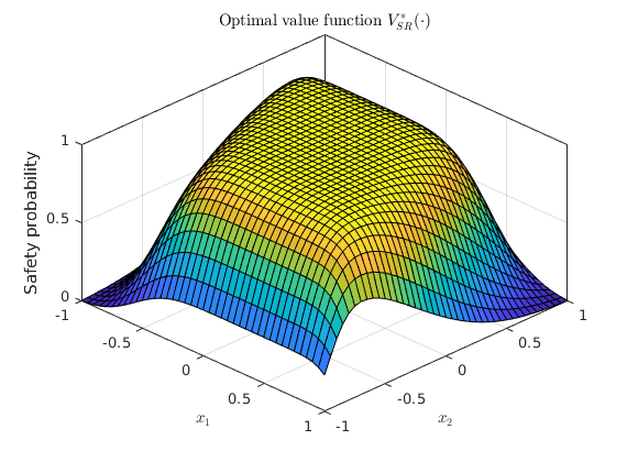
- Obtain the dynamic programming solution via SReachDynProg
- Obtain the stochastic viability sets at desired thresholds using getDynProgLevelSets2D
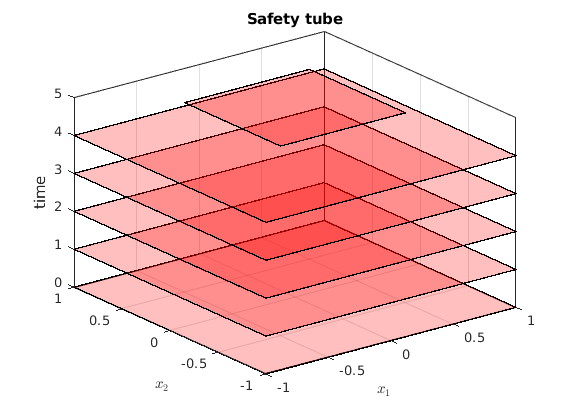
% Safety tube definition
% ----------------------
% time horizon
N = 5;
% The viability problem is equivalent to a stochastic reachability of a target
% tube of repeating safe sets
safe_set = Polyhedron('lb', [-1, -1], 'ub', [1, 1]);
safety_tube1 = Tube('viability', safe_set, N);

% Plotting of safety tube
% -----------------------
figure()
hold on
for time_indx = 0:N
    % Embed the 2-D safety sets in a 3-D space which is state-space x [0, N]
    safety_tube_at_time_indx = Polyhedron('H', ...
        [safety_tube1(time_indx+1).A, ...
            zeros(size(safety_tube1(time_indx+1).A,1),1), ...
            safety_tube1(time_indx+1).b], ...
        'He',[0 0 1 time_indx]);
    plot(safety_tube_at_time_indx, 'alpha',0.25);
end
axis([axis_vec 0 N])
box on;
grid on;
xlabel('$x_1$','interpreter','latex');
ylabel('$x_2$','interpreter','latex');
zlabel('time');
title('Safety tube');
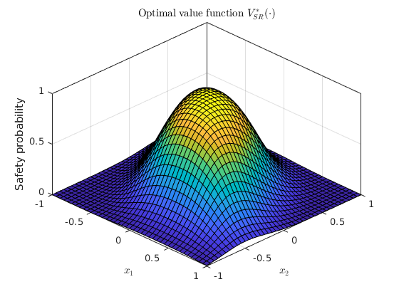
% Dynamic programming recursion via gridding
% ------------------------------------------
tic;
[prob_x1, cell_of_xvec_x1] =  SReachDynProg('term', sys, dyn_prog_xinc, ...
    dyn_prog_uinc, safety_tube1);
toc

% Plotting of the optimal value function
% --------------------------------------
% Visualization of the value function at k=0 (safety probability)
figure();
x1vec = cell_of_xvec_x1{1};
x2vec = cell_of_xvec_x1{2};
surf(x1vec,x2vec,reshape(prob_x1,length(x2vec),length(x1vec)));
axis([axis_vec 0 1])
xlabel('$x_1$','interpreter','latex');
ylabel('$x_2$','interpreter','latex');
zlabel('Safety probability')
title('Optimal value function $V_{SR}^\ast(\cdot)$','interpreter','latex');
box on
view(45, 45)
Elapsed time is 18.495988 seconds.
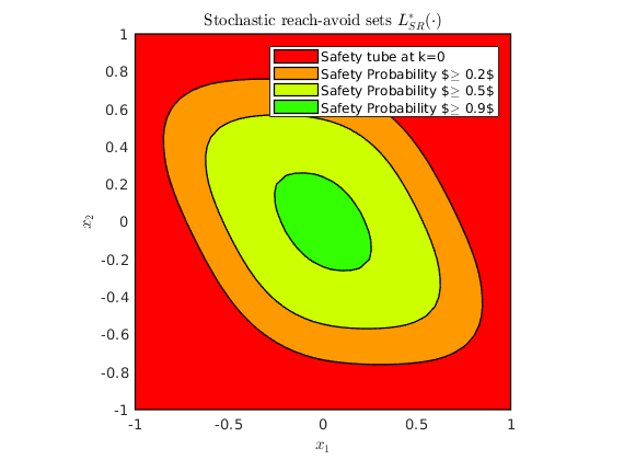
% Obtain the stochastic viability sets
% ------------------------------------
poly_array1 = getDynProgLevelSets2D(cell_of_xvec_x1, prob_x1, ...
    reach_set_thresholds, safety_tube1);

% Plotting of the stochastic viability sets
% -----------------------------------------
% Visualization of the safe initial states --- Superlevel sets of safety
% probability
figure();
hold on;
plot([safety_tube1(1), poly_array1])
xlabel('$x_1$','interpreter','latex');
ylabel('$x_2$','interpreter','latex');
box on
axis(axis_vec)
axis equal
legend(legend_str)
title('Stochastic viability sets $L_{SR}^\ast(\cdot)$','interpreter','latex');
Warning: MATLAB's contour matrix missed a corner!
Adding (1, -1) to polytope vertex list for level=0.20.
Warning: MATLAB's contour matrix missed a corner!
Adding (-1, 1) to polytope vertex list for level=0.20.
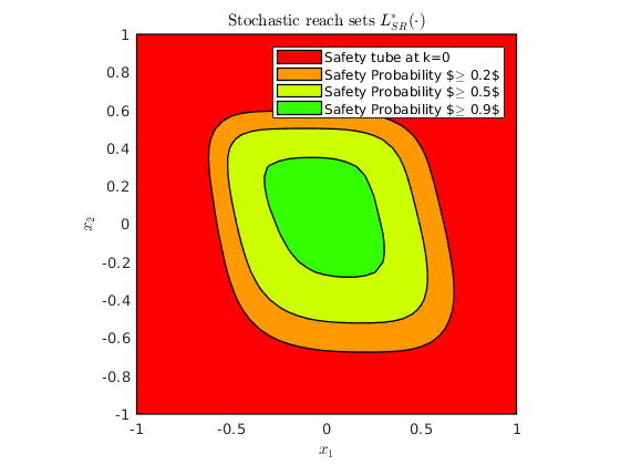
Case 2: Terminal hitting-time stochastic reach-avoid
Stochastic reach-avoid problems have a time-invariant safety set uptil time horizon (uptill  ), and a different target set at time horizon
  .
.
Specifically, we are interested in assessing the safety of this double integrator system to stay within the safe set of for  time steps and then reach
 ![$[-0.5,0.5]^2$](dIntSReachDyn_eq05409236955776165217.png) . Here, the car at has some initial position and velocity in as before.
. Here, the car at has some initial position and velocity in as before.
To perform this safety analysis, we need to do the following steps
- Provide parameters for dynamic programming like grid size and thresholds (if stochastic reach-avoid sets are of interest) [*Reused from above*]
- Construct the safety tube using 'reach-avoid' option (and plot it as well)
- Obtain the dynamic programming solution via SReachDynProg
- Obtain the stochastic reach-avoid sets at desired thresholds using getDynProgLevelSets2D
% Safety tube definition
% ----------------------
% Safety tube is a generalization of the reach problem. The reach avoid
% safety-tube is created by setting the first $N$ sets in the tube as the
% |safe_set| and the final set as the |target_set|.
%
% time horizon
N = 5;
% The viability problem is equivalent to a stochastic reachability of a target
% tube of repeating safe sets
safe_set = Polyhedron('lb', [-1, -1], 'ub', [1, 1]);
target_set = Polyhedron('lb', [-0.5, -0.5], 'ub', [0.5, 0.5]);
safety_tube2 = Tube('reach-avoid', safe_set, target_set, N);

% Plotting of safety tube
% -----------------------
figure()
hold on
for time_indx = 0:N
    % Embed the 2-D safety sets in a 3-D space which is state-space x [0, N]
    safety_tube_at_time_indx = Polyhedron('H', ...
        [safety_tube2(time_indx+1).A, ...
            zeros(size(safety_tube2(time_indx+1).A,1),1), ...
            safety_tube2(time_indx+1).b], ...
        'He',[0 0 1 time_indx]);
    plot(safety_tube_at_time_indx, 'alpha',0.25);
end
axis([axis_vec 0 N])
box on;
grid on;
xlabel('$x_1$','interpreter','latex');
ylabel('$x_2$','interpreter','latex');
zlabel('time');
title('Safety tube');
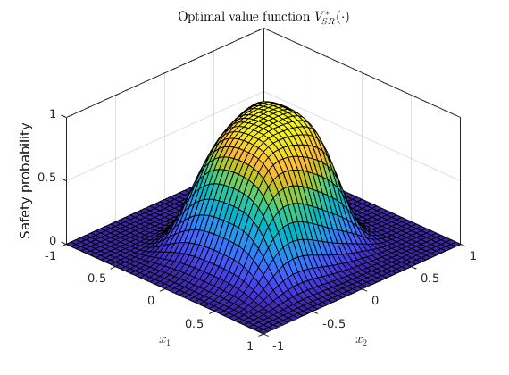
% Dynamic programming recursion via gridding
% ------------------------------------------
tic;
[prob_x2, cell_of_xvec_x2] =  SReachDynProg('term', sys, dyn_prog_xinc, ...
    dyn_prog_uinc, safety_tube2);
toc
% Plotting of the optimal value function
% --------------------------------------
% Visualization of the value function at k=0 (safety probability)
figure();
x1vec = cell_of_xvec_x2{1};
x2vec = cell_of_xvec_x2{2};
axis([axis_vec 0 N]);
surf(x1vec,x2vec,reshape(prob_x2,length(x2vec),length(x1vec)));
xlabel('$x_1$','interpreter','latex');
ylabel('$x_2$','interpreter','latex');
zlabel('Safety probability')
box on
view(45, 45)
title('Optimal value function $V_{SR}^\ast(\cdot)$','interpreter','latex');
Elapsed time is 19.003879 seconds.
% Obtain the stochastic reach-avoid sets
% --------------------------------------
poly_array2 = getDynProgLevelSets2D(cell_of_xvec_x2, prob_x2, ...
    reach_set_thresholds, safety_tube2);

% Plotting of the stochastic reach-avoid sets
% -------------------------------------------
% Visualization of the safe initial states --- Superlevel sets of safety
% probability
figure();
hold on;
plot([safety_tube2(1) poly_array2])
box on
xlabel('$x_1$','interpreter','latex');
ylabel('$x_2$','interpreter','latex');
axis(axis_vec);
box on
axis equal
legend(legend_str)
title('Stochastic reach-avoid sets $L_{SR}^\ast(\cdot)$','interpreter','latex');
Case 3: Time-varying safety sets (Stochastic reachability of a target tube)
Stochastic reachability of a target tube has time-varying safety sets.
To perform this safety analysis, we need to do the following steps
- Provide parameters for dynamic programming like grid size and thresholds (if stochastic reach sets are of interest) [*Reused from above*]
- Construct the safety tube by constructing at piecemeal (and plot it as well)
- Obtain the dynamic programming solution via SReachDynProg
- Obtain the stochastic reach sets at desired thresholds using getDynProgLevelSets2D
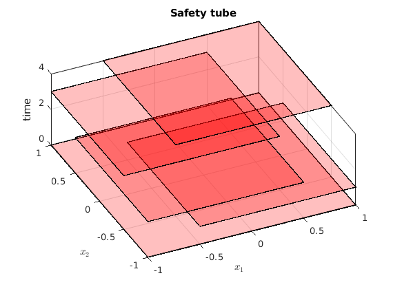
% Safety tube definition
% ----------------------
safety_tube3 = Tube(Polyhedron('lb', [-1, -1], 'ub', [1, 1]), ...
    Polyhedron('lb', [-0.5, -1], 'ub', [1, 0.5]), ...
    Polyhedron('lb', [-1, -1], 'ub', [0.5, 0.5]), ...
    Polyhedron('lb', [-1, -0.5], 'ub', [0.5, 1]), ...
    Polyhedron('lb', [-0.5, -0.5], 'ub', [1, 1]));
N = length(safety_tube3)-1;

% Plotting of safety tube
% -----------------------
figure()
hold on
for time_indx = 0:N
    % Embed the 2-D safety sets in a 3-D space which is state-space x [0, N]
    safety_tube_at_time_indx = Polyhedron('H', ...
        [safety_tube3(time_indx+1).A, ...
            zeros(size(safety_tube3(time_indx+1).A,1),1), ...
            safety_tube3(time_indx+1).b], ...
        'He',[0 0 1 time_indx]);
    plot(safety_tube_at_time_indx, 'alpha',0.25);
end
axis([axis_vec 0 N])
box on;
grid on;
xlabel('$x_1$','interpreter','latex');
ylabel('$x_2$','interpreter','latex');
zlabel('time');
title('Safety tube');
view([-25 60]);
% Dynamic programming recursion via gridding
% ------------------------------------------
tic;
[prob_x3, cell_of_xvec_x3] =  SReachDynProg('term', sys, dyn_prog_xinc, ...
    dyn_prog_uinc, safety_tube3);
toc
% Plotting of the optimal value function
% --------------------------------------
% Visualization of the value function at k=0 (safety probability)
figure();
x1vec = cell_of_xvec_x3{1};
x2vec = cell_of_xvec_x3{2};
axis([axis_vec 0 N]);
surf(x1vec,x2vec,reshape(prob_x3,length(x2vec),length(x1vec)));
xlabel('$x_1$','interpreter','latex');
ylabel('$x_2$','interpreter','latex');
zlabel('Safety probability')
box on
view(45, 45)
title('Optimal value function $V_{SR}^\ast(\cdot)$','interpreter','latex');
Elapsed time is 10.287044 seconds.
% Obtain the stochastic reach sets
% --------------------------------
poly_array3 = getDynProgLevelSets2D(cell_of_xvec_x3, prob_x3, ...
    reach_set_thresholds, safety_tube3);

% Plotting of the stochastic reach sets
% -------------------------------------
% Visualization of the safe initial states --- Superlevel sets of safety
% probability
figure();
hold on;
plot([safety_tube3(1) poly_array3])
box on
xlabel('$x_1$','interpreter','latex');
ylabel('$x_2$','interpreter','latex');
axis(axis_vec);
box on
axis equal
legend(legend_str)
title('Stochastic reach sets $L_{SR}^\ast(\cdot)$','interpreter','latex');